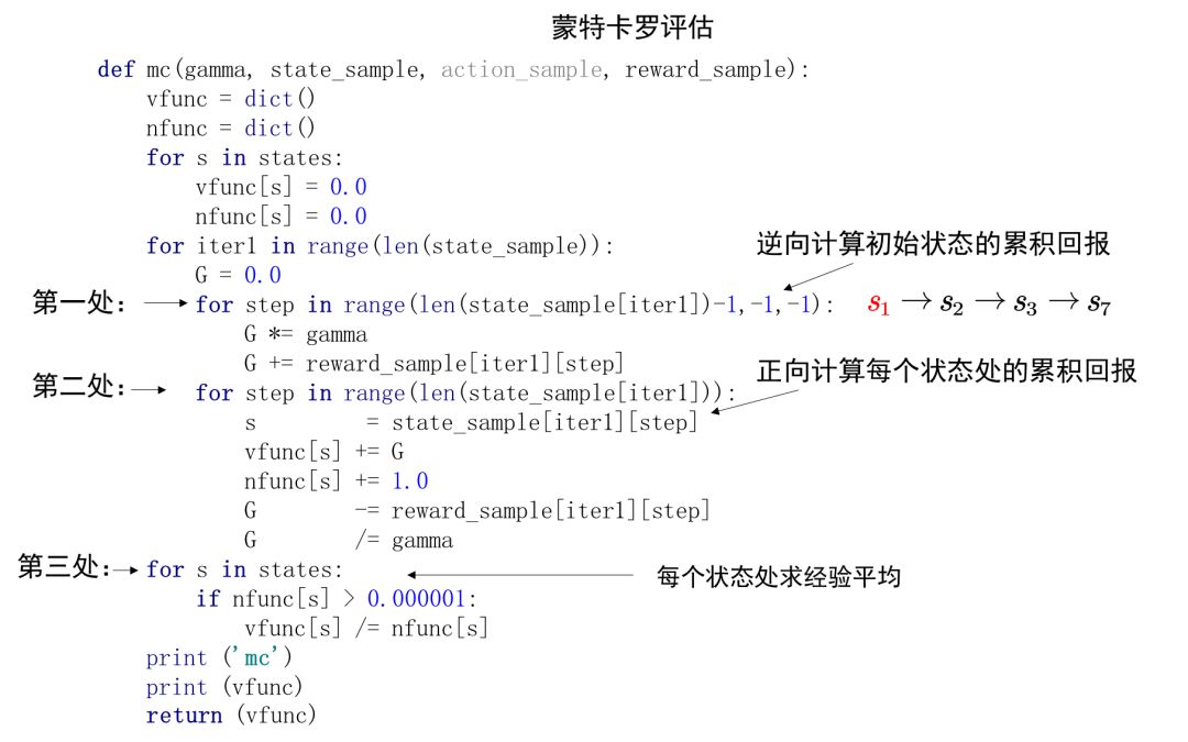
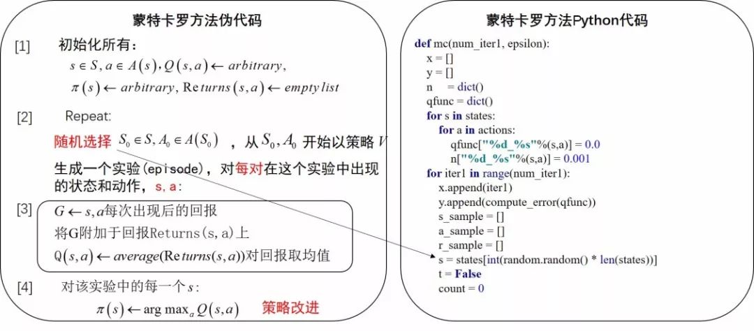
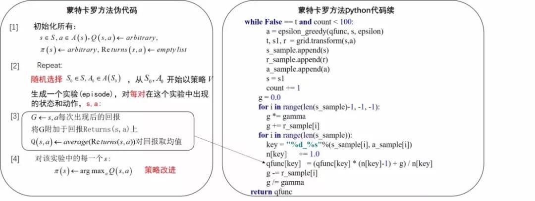
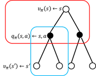
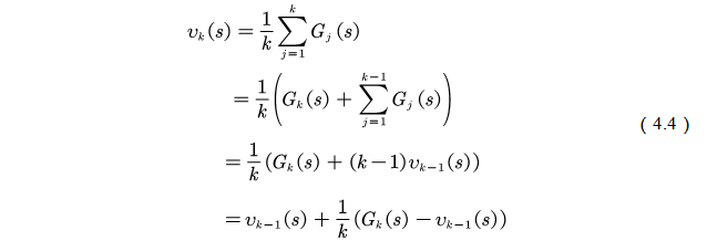
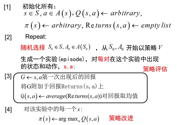
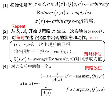
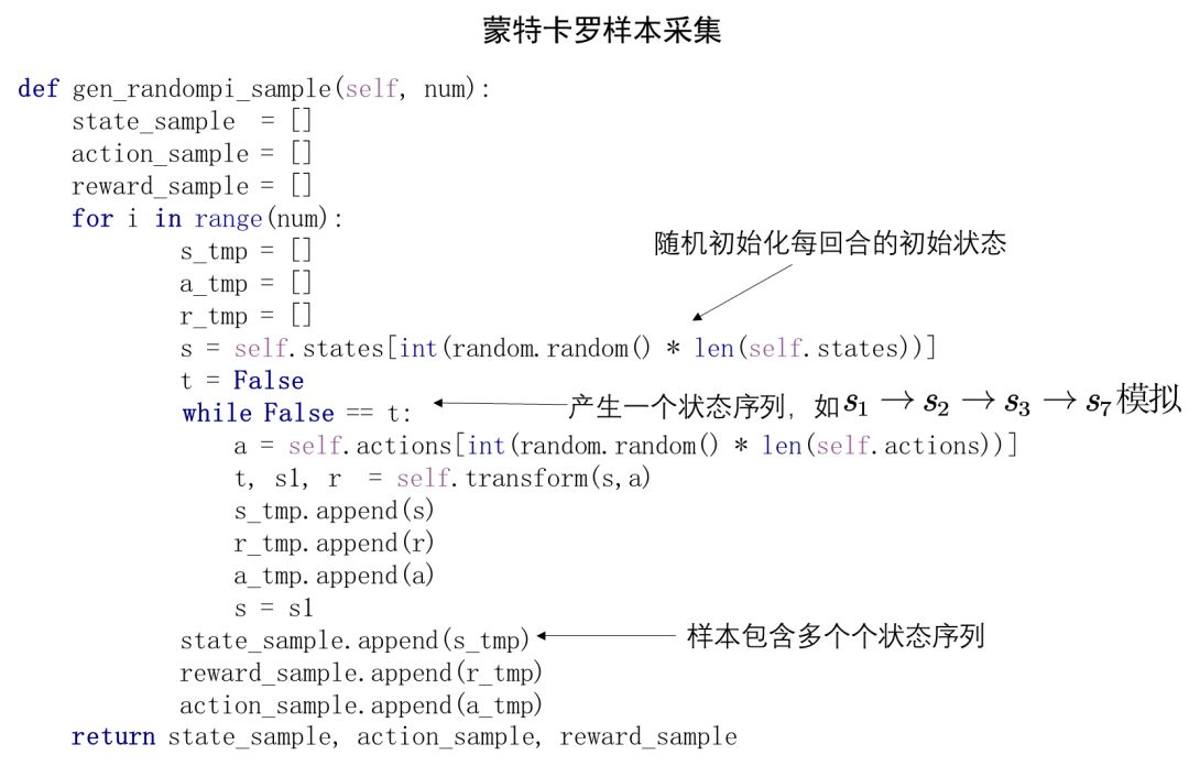
â–Œ4.1 Theory based on Monte Carlo method In this chapter we study the model-free reinforcement learning algorithm. One of the essence of the reinforcement learning algorithm is to solve the Markov decision problem without model. As shown in Figure 4.1, the model-free reinforcement learning algorithm mainly includes Monte Carlo method and time difference method. In this chapter we describe the Monte Carlo method. Figure 4.1 Classification of reinforcement learning methods Before learning the Monte Carlo method, we will sort out the research ideas of reinforcement learning. First, the reinforcement learning problem can be incorporated into the Markov decision process, and this knowledge is covered in Chapter 2. In the case of known models, the dynamic programming approach can be used (the idea of ​​dynamic programming is the root of no-model reinforcement learning research, so focus on) to solve the Markov decision process. Chapter 3 describes two methods of dynamic programming: policy iteration and value iteration. These two methods can be unified by the generalized strategy iterative method: first, the strategy evaluation is performed, that is, the value function corresponding to the current strategy is calculated, and then the value function is used to improve the current strategy. The same is true of the basic idea of ​​model-free reinforcement learning, namely: strategy evaluation and strategy improvement. In the dynamic programming method, the calculation method of the value function is shown in Figure 4.2. Figure 4.2 Value function calculation method The dynamic programming method utilizes the model when calculating the value function at state s We return to the most primitive definition of the value function (see Chapter 2): The calculation of the state value function and the behavior value function is actually the expectation of calculating the return value (see Figure 4.2). The method of dynamic programming is to use the model to calculate the expectation. In the absence of a model, we can use Monte Carlo's method to calculate this expectation, using random samples to estimate expectations. When calculating the value function, the Monte Carlo method is the expectation of using the empirical average instead of the random variable. Here we have to understand two words: experience and average. First look at what is "experience." When we want to evaluate the current strategy of the agent, we can use the strategy to generate many experiments, each test starts from any initial state until the end, such as an episode Figure 4.3 Experience in Monte Carlo Let’s see what is “averageâ€. The concept is simple, and the average is to find the mean. However, when using the Monte Carlo method to find the value function at the state, it can be divided into the first access Monte Carlo method and each visit to the Monte Carlo method. The first visit to the Monte Carlo method means that when calculating the value function at the state, only the return value when the state s is accessed for the first time in each test is utilized. As shown in the first test in Figure 4.3, only the mean at the state s is used. Each visit to the Monte Carlo method refers to the return value of the return when all values ​​are accessed to the state s when calculating the value function at state s, ie According to the law of large numbers: Since the model of the interaction between the agent and the environment is unknown, the Monte Carlo method uses the empirical average to estimate the value function, and whether the correct value function can be obtained depends on the experience – therefore, how to obtain sufficient experience is no model. The core of intensive learning. In the dynamic programming method, in order to ensure the convergence of the value function, the algorithm scans the state in the state space one by one. The model-free approach to fully evaluate the strategy value function assumes that each state can be accessed. Therefore, in the Monte Carlo method, certain methods must be used to ensure that each state can be accessed. One of the methods is exploratory. initialization. Exploratory initialization means that each state has a certain probability as an initial state. Before learning the Monte Carlo method based on exploratory initialization, we also need to understand the strategy improvement method and the average method for iterative calculation. Below we introduce the Monte Carlo strategy improvement method and the method of incrementally calculating the mean. (1) Monte Carlo strategy improvement. The Monte Carlo method utilizes an empirical average to estimate the strategy value function. After estimating the value function, for each state s, it improves the strategy by maximizing the action value function. which is (2) The method of incrementally calculating the mean is as shown in equation (4.4). As shown in Figure 4.4, the pseudo code for exploratoryly initializing the Monte Carlo method is noted. First, in the second step, the initial state and action of each test are random to ensure that each state behavior pair has an opportunity as an initial state. When evaluating the state behavior value function, it is necessary to estimate all state behavior pairs in each trial; Second, step 3 completes the strategy assessment and step 4 completes the strategy improvement. Figure 4.4 Exploratory Initialization Monte Carlo Method Let's talk about exploratory initialization. Exploratory Initialization At the time of iterating each scene, the initial state is randomly assigned, which ensures that each state behavior pair can be selected during the iteration. It implies a hypothesis: assume that all actions are selected infinitely frequently. This assumption is sometimes difficult to establish or cannot be fully guaranteed. We will ask, how to ensure that each state behavior pair can be accessed while the initial state is unchanged? A: Carefully design your exploration strategy to ensure that every state is accessible. But how do you carefully design your exploration strategy? What should be the search strategy that meets the requirements? A: The strategy must be moderate, that is, satisfy all states s and a: According to whether the exploration strategy (action strategy) and the evaluated strategy are the same strategy, the Monte Carlo method is divided into two methods: on-policy and off-policy. If the action strategy and the assessment and improvement strategy are the same strategy, we call it on-policy and can be translated into the same strategy. If the action strategy and the strategy of assessment and improvement are different strategies, we call it off-policy and can be translated into a different strategy. Next we focus on the on-policy method and the off-policy method. (1) The same strategy. On-policy means that the strategy for generating data is the same strategy as the assessment and the strategy to be improved. For example, the strategies and assessments to generate data and the strategies to be improved are Figure 4.5 The same strategy Monte Carlo reinforcement learning method The strategies for generating data in Figure 4.5, as well as the strategies for evaluation and improvement, are (2) Different strategies. Off-policy means that the strategy for generating data is not the same strategy as the strategy for evaluating and improving. we use Different strategies can ensure full exploratoryness. For example, strategies for evaluation and improvement Target strategy for different strategies Using data generated by behavioral strategies to evaluate target strategies requires the use of importance sampling methods. Below, we introduce importance sampling. We use Figure 4.6 to describe the principle of importance sampling. The importance of sampling comes from the expectation, as shown in Figure 4.6: Figure 4.6 Importance sampling As shown in Figure 4.6, when the distribution of the random variable z is very complicated, it is impossible to use the analytical method to generate the sample for approximating the expectation. In this case, we can choose a probability distribution that is very simple and easily generate the probability distribution of the sample. Define importance weights: From equation (4.7), the integral estimate based on the importance sample is an unbiased estimate, ie the estimated expectation is equal to the true expectation. However, the variance of the integral estimate based on importance sampling is infinite. This is because the original integrand multiplied by an importance weight, changing the shape and distribution of the integrand. Although the mean of the integrand did not change, the variance changed significantly. In importance sampling, the closer the sampling probability distribution is to the original probability distribution, the smaller the variance. However, the probability distribution of the integrand is often difficult to find, or very strange, so there is no similar simple sampling probability distribution. If the original probability distribution is sampled using sampling probabilities with widely different distributions, the variance will approach gigantic. One way to reduce the variance of importance sampling is to use weighted importance sampling: Action strategy in a different strategy approach Target strategy In action strategy Therefore, the importance weight is (4.10) The value function of the ordinary importance sample is estimated as shown in Figure 4.7: Figure 4.7 General importance sampling calculation formula The specific meaning of each symbol in the formula (4.11) will now be illustrated. As shown in FIG. 4.8, t is the time at which the state s is accessed, and T(t) is the time corresponding to the termination state of the test corresponding to the access state s. T(s) is the set of all times at which the state s occurs. In this case, Figure 4.8 Example of importance sampling formula The weighted importance sample value function is estimated as Finally, we give the pseudo-code for each visit to the Monte Carlo algorithm, as shown in Figure 4.9. Figure 4.9 Monte Carlo method pseudo code Note: Soft strategy here To sum up: This section focuses on how to use the MC method to estimate the value function. Compared with the dynamic programming-based method, the MC-based method only differs in the value function estimation, and is the same in the whole framework, that is, the current strategy is evaluated, and the learned value function is used to improve the strategy. This section needs to focus on understanding the concepts of on-policy and off-policy, and learn to use importance sampling to evaluate the value function of the target strategy. â–Œ4.2 Basic knowledge of statistics Why do you want to talk about statistics? Let's take a look at the definition of statistics. Statistics is about the science of data. It provides a set of methods for collecting, processing, analyzing, interpreting, and drawing conclusions from data. Contact us about the concept of reinforcement learning algorithms: Reinforcement learning is the process by which an agent interacts with the environment to generate data and internalizes the knowledge it learns into its own behavior. The process of learning is actually the processing and processing of data. In particular, the estimation of the value function is a process of estimating the true value using data, involving sample mean, variance, biased estimation, etc. These are statistical terms. Here's a brief introduction. Overall: Contains a collection of all the data studied. Sample: A collection of a subset of elements extracted from the population. In episode reinforcement learning, a sample refers to a scene of data. Statistics: A generalized numerical measure used to describe sample characteristics. Such as sample mean, sample variance, sample standard deviation, etc. In reinforcement learning, we measure the state value function with the sample mean. Sample mean: Assume The sample mean is also a random variable. Sample variance: Assume Unbiased estimation: If the statistic of the sample is equal to the statistic of the population, the statistic corresponding to the sample is said to be an unbiased estimate. If the overall mean and variance are Monte Carlo integral and random sampling method [3]: The Monte Carlo method is often used to calculate the integral of a function, such as calculating the integral of the following formula. If the functional form of f(x) is very complex, then (4.13) cannot apply parsed form calculations. At this time, we can only use the numerical method to calculate. Using the numerical method to calculate the integral of (4.13) requires taking a number of sample points, calculating the values ​​of f(x) at these sample points, and averaging these values. So the question is: How do you take these sample points? How to average the function values ​​at the sample points? For these two problems, we can convert the (4.13) equivalent to among them Question 1: How to sample this point? A: Because Question 2: How to average? A: According to the distribution The above is the principle of calculating the integral using the Monte Carlo method. Let's take a look at the expected calculations. Let X denote a random variable and obey the probability distribution Using Monte Carlo's method to calculate this formula is very simple, that is, constantly distributed from However, when the target is distributed There are two types of commonly used sampling methods. The first type is to specify a known probability distribution. (1) Refusal to sample. Target distribution (2) Importance sampling. Importance sampling We have already made a more detailed introduction in Section 4.1. (3) MCMC method. The MCMC method is considered the algorithm of the twentieth century Top 10. The MCMC method is called the Markov chain Monte Carlo method. When the dimension of the sampling space is relatively high, rejection sampling and importance sampling are not practical. The principle of MCMC sampling is fundamentally different from the principle of rejecting sampling and importance sampling. Rejection sampling and importance sampling use the proposed distribution to generate sample points. When the dimension is high, it is difficult to find a suitable distribution of proposals, and the sampling efficiency is poor. The MCMC method does not need to propose a distribution, only a random sample point is needed, and the next sample will be generated by the current random sample point, so that the loop continuously generates many sample points. Ultimately, these sample points obey the target distribution. How do you generate the next sample point from the current sample point and ensure that the sample thus produced obeys the original target distribution? The theorem behind it is that the target distribution is a stable distribution of Markov chains. So, what is the stable distribution of the Markov chain? Simply put, there is a transition probability matrix for the target distribution, and the transition probability satisfies: Transfer matrix Now the problem is transformed into finding the transition probability corresponding to the target distribution. The transition probability and distribution should satisfy the meticulous stability conditions. So-called smooth condition, ie Next, how to construct a transition probability using careful balance conditions? We can consider this: adding an existing Markov chain whose transfer matrix is ​​Q, so that the arbitrarily selected transfer matrix usually does not satisfy the fine balance condition, that is, Since it is not satisfied, we can transform The question is how to take Which is called the acceptance rate. The MCMC sampling algorithm can be summarized as the following steps. 1 Initialize the initial state of the Markov chain 2 pairs 3 The Markov chain state at time t is 4 sampling from a uniform distribution 5 if 6 Otherwise, no transfer will be accepted, ie In order to increase the acceptance rate and diversify the sample, the acceptance rate of the MCMC line 5 can usually be rewritten as â–Œ4.3 Python-based programming examples In this section, we use Python and Monte Carlo methods to solve the problem of robots looking for gold coins. The Monte Carlo method solves the problem of reinforcement learning without models. The basic idea is to use the experience average to replace the expectation of random variables. Therefore, using the Monte Carlo method to evaluate a strategy should include two processes: simulation and averaging. The simulation is to generate sampled data, and the average is to obtain a value function based on the data. Below we take the Monte Carlo method to estimate the value function of the stochastic strategy as an example. 1. Sample generation of stochastic strategies: simulation Figure 4.10 shows the sampling process for the Monte Carlo method. The sampling function consists of two large loops, the first large loop representing the sampling of multiple sample sequences and the second loop representing the generation of each specific sample sequence. It should be noted that the initial state of each sample sequence is random. Because the evaluation is a random and evenly distributed strategy, at the time of sampling, the actions are generated according to a random function. Each sample sequence includes a sequence of states, a sequence of actions, and a sequence of rewards. Figure 4.10 Monte Carlo sample acquisition Figure 4.11 shows the Python code implementation for policy evaluation for the Monte Carlo method. There are three places where the function needs to be explained. The first place: inversely calculate the cumulative return at the initial state of the sequence for each simulation sequence, that is, calculate from the last state of the sequence, and finally obtain the cumulative return at the initial state. The second place: Calculate the cumulative function corresponding to each state in the forward direction, and calculate the formula as . The third place: the average, that is, the cumulative and average of the number of occurrences of the state. Corresponds to each visit to the Monte Carlo method in Section 1. The Python code in Figure (4.10) and Figure (4.11) combine to form an evaluation method based on Monte Carlo method. Below, we implement a Monte Carlo-based reinforcement learning algorithm. The pseudo code of the Monte Carlo method is shown in Figure 4.12 and Figure 4.13, where the key code is implemented in Figure 4.13. Comparing Figure 4.13 with Monte Carlo Strategy Evaluation Figure 4.11, we can easily find that Monte Carlo reinforcement learning evaluates every iteration. Figure 4.11 Monte Carlo Strategy Assessment The Python implementation of the Monte Carlo reinforcement learning algorithm is shown in Figure 4.12 and Figure 4.13. Figure 4.12 Monte Carlo method pseudo code and Python code Figure 4.13 Monte Carlo method pseudo code and Python code Shenzhen Ruidian Technology CO., Ltd , https://www.wisonens.com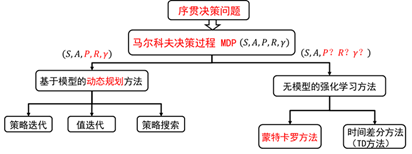

 In model-free reinforcement learning, the model
  It is unknown. Model-Free Reinforcement Learning Algorithms To take advantage of the framework of policy evaluation and policy improvement, other methods must be used to evaluate the current strategy (calculated value function).
 Calculate the return value of the discount return at the state in one test
  Then "experience" means using this strategy to do many experiments and generate a lot of screen data (the scene here is the meaning of a test), as shown in Figure 4.3.
 , so the calculation formula for the first visit to the Monte Carlo method is
 ,
,  .
. 
 . That is to say, the gentle exploration strategy means that in any state, the probability of using each action in the action set is greater than zero. A typical mild strategy is
  Strategy:
 Strategy. Its pseudo code is shown in Figure 4.5.
 Strategy.
  Represents strategies for evaluation and improvement,
  Represents the strategy for generating sample data.
  Is a greedy strategy, an exploratory strategy for generating data
  For exploratory strategies, such as
  Strategy.
  And action strategy
  It is not arbitrarily chosen, but must meet certain conditions. This condition is the coverage condition, ie the action strategy
  The resulting behavior covers or contains the target strategy
  The resulting behavior. Use the expression of the formula: satisfied
  any
any  All satisfied
  .
. 
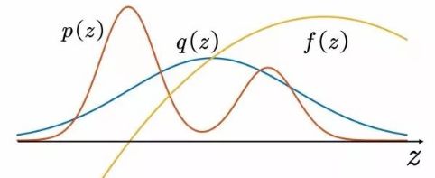
 , such as a normal distribution. The original expectation can be changed to
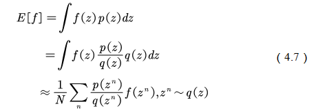
 , the ordinary importance of sampling and integration is as shown in equation (4.7)

 The strategy used to generate the sample, the resulting trajectory probability distribution is equivalent to the importance sample
  , strategies for evaluation and improvement
  The corresponding trajectory probability distribution is
  So using action strategies
  The resulting cumulative function return value to evaluate the strategy
  When you want to multiply the importance weight in front of the cumulative function return value.
  Next, the probability of one trial is
 Next, the probability of the corresponding test is

 (4.11)
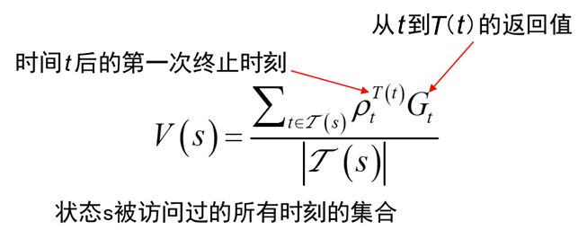


 (4.12)
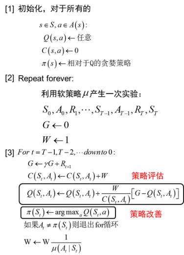
 for
for  Strategy, strategy that needs improvement
  For greedy strategies.
  For random samples with a sample size of n, they are independent and identically distributed random variables, and the sample mean is
  ,
,  For random samples with a sample size of n, they are independent and identically distributed random variables, and the sample variance is
 with
with  When, if
  ,then
,then  with
with  It is called unbiased estimation.
  (4.13)
  (4.14)
  Is a known distribution. After transforming the equation (4.13) into the equivalent (4.14), we can answer the above two questions.
  Is a distribution, so random sampling can be performed according to the distribution to obtain sampling points.
  .
.  sampling
  After calculating at the sample point
  And average the values ​​at all sample points:
  (4.15)
 , calculation function
 Expectations. function
  The expected calculation formula is
 Sampling
  And then to these
  Average by approximation
  Expectations. This is also the method of estimating the function in Section 4.1. Only one sample there is an episode, each episode produces a state value function, and Monte Carlo's method estimates the state value function by summing the state value functions at these sample points for averaging, which is the empirical average.
  When it is very complicated or unknown, we can't get the sampling points of the target distribution. If we can't get the sampling points, we can't calculate (4.15), and we can't calculate the average. At this time, we need to use various sampling techniques in statistics.
  For sampling, the specified sampling probability distribution is called the proposed distribution. This type of sampling method includes rejection of sampling and importance sampling. Such methods are only suitable for low-dimensional cases, and for the high-dimensional case, the second type of sampling method, that is, the Markov chain Monte Carlo method is often used. The basic principle of the method is to generate non-independent samples from a smoothly distributed Markov chain. Below we briefly introduce these methods.
  When it is very complicated or unknown, it is impossible to give a sampling point using the target distribution. What should I do? One way is to use a distribution that is easy to sample.
  , such as Gaussian distribution for sampling. However, if the distribution is proposed
  Sampling, then the resulting sample is subject to the proposed distribution
  Disobeying target distribution
  . So, in order to get the target distribution
  Sample, need to be processed by the proposed distribution
  The sample obtained. Receive samples that match the target distribution and reject samples that do not match the target distribution.
 Is the equation
  The only non-negative solution.
  Any initial distribution from the above conditions
  Departure, after a period of iteration, distribution
  Will converge to the target distribution
  . Therefore, suppose we already know the state transition probability matrix that satisfies the condition.
  , then we just have to give any initial state
 , you can get a transfer sequence
 . If the Markov chain has converged to the target distribution at the nth step
  Then we get a sample that obeys the target distribution
  .
.  So how do you construct a transition probability?

 To make it satisfy. The method of transformation is to add one
 What? A simple idea is to take advantage of the symmetry of the expression, ie
 ;
;  , loop 3~6 below, continue sampling;
  ,sampling;
  ;
;  , accept the transfer
  , the state of the next moment
  ;
;  .
.  The algorithm for sampling this acceptance rate is called the Metropolis- Hastings algorithm.
 , the calculation formula is
 Strategy.